ELMAG-2D
TERMS AND DEFINITIONS
Point – is a place of intersection of neighboring boundaries of one body or a separately set point.
Boundary – is a straight line or a circle (a part of a circle), determining a boundary of the body.
Body – is a set of boundaries, forming a closed space; with each such space (body) a definite property associates.
Property – is a set of data, determining parameters of problem, body material, circuit and boundary conditions.
Block – is a separately set label with special properties; block sets up relation between the body and the property.
MAKE-UP OF THE SOFTWARE
The software is a separate executable module, operating under the operating systems WINDOWS 98, NT, 2000, XP. In single software input of initial data, calculation and review of calculation results is made.
The software consists of a set of windows, in which the user makes input of initial data, execution of calculations, reviewing results.
Initial data of the problem are conventionally divided into two parts: geometric bodies and their physical properties. Each part of initial data is connected with a file: file with *.scn extension comprises geometry information of the problem, file with *.hlm extension comprises physical properties information.
After execution of calculations the software creates a file of calculation results with .hlr extension. Software uses this file for analysis of calculation results.
All files of a sole problem should have the same names and should be in the same folder.
INPUTS OF INITIAL DATA
The software is a standard WINDOWS application. At the start the software is presented as a window, in the upper part of which there is a menu and a number of buttons, duplicating menu items. The most part of the window is occupied by the working area intended for input of geometric bodies of the problem. At the left part of the window there is a tree of properties of the problem and geometric bodies. The work with the program can be started with creation of a new problem, editing the existing one or analyzing the results of the calculated problem.
In order to create a new problem it is necessary to select the menu item «File/New».
In order to load a problem from hard disk it is necessary to select menu item «File/Open…» select the required file with *.hlm extension and load it using standard means of WINDOWS file system.
In order to load calculation results from hard disk it is necessary to select menu item «File/Open…», select the required file with .hlr extension and load it, using standard means of WINDOWS file system
Calculation model composition has two stages: geometry objects construction (see item 4.1) and properties and boundary conditions assigning (see item 4.2)
Figure 4.1 Main window of problem
Geometry object composition
A geometry object is a set of closed bodies with assigned labels with physical properties and boundary conditions. When describing model geometry one has to set points and boundaries bounding bodies of object
The main requirement in blocks boundaries specifying is that all intersections and contacts of boundaries shall be done in the points, contact or intersection of boundaries without setting the top is inadmissible, the software automatically calculates intersection of boundaries (line – line, line – segment of an arc, segment of an arc – segment of an arc).
Graphics editor interface is similar to the CAD-programs interface: it is possible to create new points and boundaries, to move, duplicate and remove any geometrical objects. For execution of the operation with several objects simultaneously, the mechanism of selection shall be used.
In addition to composition of geometry by means of graphics editor it is possible to exchange information via DXF14 file format that is supported by most computer aided design software (CAD).
When composing model geometry using CAD program with a purpose of further import to DXF format one must follow a set of conditions:
- bodies must consist only of simple lines and arcs of a circle;
- bodies must be ungrouped;
- linear dimension unit is to be millimeter;
- angular dimension unit is to be degree;
- Y-axis directed vertically upwards;
- X-axis directed horizontally from left to right;
- when composing lines and arcs of circle it is obligatory to use snap mode to points and grid nodes, grid spacing have to be enough for exact assigning of any coordinate in the model.
Geometry objects composition and assigning of properties and boundary conditions is performed in the problem main window (Fig. 4.1).
Graphics tools of problem main window
1 – Buttons: Create new problem, Open problem, Save problem, Save problem as…
2 – Buttons: Undo the last image edition operation; Redo previously canceled image edition operation.
3 – Buttons: Switch on primitive selecting mode. In order to select a group of primitives it is necessary to press left mouse button and drag mouse cursor right and down enclosing the necessary model part with frame. When the left mouse button is released all primitives enclosed with the frame will be selected.
Open the primitive copy window. This button opens the move selected primitives window (Fig. 4.2). In case of nonzero value of «Angle of rotation, degree» parameter the program rotates (copies) selected primitives around the point determined by «Move by X axis / Rotates around X» and «Move by Y axis / Rotates around Y» coordinates. In case of zero value of parameter «Angle of rotation, degree» the program moves (copies) selected primitives on vector determined by «Move by X axis / Rotates around X» and «Move by Y axis / Rotates around Y» coordinates. The «Number of copies, pcs» is enabled only on copying.
4 – Buttons: Copy image to clipboard, Print image
5 – Buttons Switch on zoom and pan mode. Zoom and Pan mode allows to perform the following actions:
- Zoom in selected image - press left mouse button and drag mouse cursor right and down enclosing the necessary model part with frame. When the left mouse button is released image inside the frame will be zoomed to fit the window. In order to return to initial scale it is necessary to press left mouse button and drag the mouse cursor left and upward.
- Pan image – press the right mouse button and drag the mouse cursor to necessary direction on necessary distance.
- Zoom in and zoom out proportionally with respect to window center – rotate mouse wheel away and toward yourself respectively
Fit model to window size, Stretch model proportionally to window width, Stretch model proportionally to window height.
Figure 4.2 The copy (move) selected primitive window
6 – Button: Switch on graphic primitive pick mode. At this mode picking the primitive is made with left mouse button.
7 – Button: Switch on point edition mode. At this mode pressing the left mouse button sets a point, pressing the right mouse button – selection.
8 – Button: Switch on line edition mode. At this mode pressing the left mouse button sets a line. The line joins two previously selected points. Pressing the right mouse button performs selection of a line.
9 – Button: Switch on arc edition mode. At this mode pressing the left mouse button sets an arc. The arc joins two previously selected points. Arc radius is assigned in the dialog window «Arc properties». Pressing the right mouse button performs selection of an arc.
10 – Button: Switch on block label edition mode. At this mode entering the label is performed by pressing the left mouse button. Pressing the right mouse button performs selection.
11 – Buttons: Zoom in, Zoom out.
14 – Buttons: Move left, Move up, Move down, Move right.
16 – Buttons: Switch on(off) snap grid visibility, Switch on(off) grid snap mode, Open the grid spacing setting dialog window.
Model properties
Model properties consist of problem properties, bodies physical properties, current sources, boundary conditions. Model properties are assigned in the tree of properties (Fig. 4.1, label 17). The tree of properties consists of four branches: problem description, block property, boundary condition, current sources parameters. Every branch of tree of properties (except for model properties) can contain unrestricted number of leaves. Leave corresponds to one property parameter (material, current source, boundary condition…).
In order to create new property (boundary condition, current source) it is necessary to set the cursor at the tree branch «Block Properties» («Boundary Condition», «Source Parameters») call the contextual menu by pressing left mouse button and select menu item «Add Block Property» («Add Boundary Condition», «Add Source Parameter»).
In order to delete block property (boundary condition, current source) it is necessary to set the cursor at the correspondent block property (boundary condition, current source) call the contextual menu by pressing left mouse button and select menu item «Delete Block Property» («Delete Boundary Condition», «Add Source Parameter»).
Parameters of the selected block property (boundary condition) can be edited in the property list (Fig. 4.1, label 18).
Model properties list
The «Problem Description» list:
Problem Type: possesses values:
Magnetic Field Of DC: calculation of nonlinear anisotropic magnetic field of direct current;
Magnetic Field Of AC: calculation of magnetic field of sinusoidal currents;
Temperature Field: calculation of temperature field;
Coupled Problem: coupled problem of magnetic field of sinusoidal currents and temperature field calculation;
Model Class: type of two-dimensional problem. Possesses values:
Planar;
Axisymmetric;
Frequency, Hz: current source frequency (applicable for problems of magnetic field of sinusoidal currents calculation);
Bodies Depth, mm: bodies length along Z-axis (applicable for planar problems);
Solver Precision: relative error of equations system solving method;
SSE2 Support: CPU SSE2 instructions support. This feature is applied for acceleration of magnetic field of sinusoidal current calculation problems. Option is supported by Windows 2000/XP operational systems and Intel-compatible CPU starting with Pentium III.
The «Block Properties» list:
Block Name: any set of symbols identifying the given block, except for the word «None».
mx, my: XX and YY components of the relative permeability tensor;
sigma, MS/m: block material conductivity;
Lambda X, Lambda Y, W/C*m: XX and YY components of the heat conductivity tensor;
B(H) Curve: this button shows magnetization curve edit window (Fig. 4.3):
«Add» button adds row for values input.
«Delete» button deletes the last row.
«Clear» button clears the entire list.
«Draw» button redraws the image.
«Import» button loads B(H) curve from a text file.
«Export» button saves B(H) curve to a text file.
«t * 1e6» textbox is intended for anisotropy factor assignment.
«Rolling Type» textbox is intended for choosing anisotropy axis.
«NMax» textbox is intended for restriction of B(H) curve nodes output.
Figure 4.3. Magnetization curve edit window
The «Boundary Condition» list
Boundary Name: any set of symbols identifying the given boundary, except for the word «None».
Flux Direction: boundary condition for magnetic problems (applied for outer boundary in magnetic field calculation problem)
Flux Parallel: magnetic flux is parallel to the boundary;
Flux Noraml: magnetic flux is normal to the boundary;
alpha, W/K*m^2: convection coefficient;
A, K
B, K/mm
C, K/mm: ambient temperature, as a function of coordinates:
t(x, y) = A + B * x + C * y
The «Source Parameters» list:
Source Name: any set of symbols identifying the given current source, except for the word «None»;
Total Current, А: current source magnitude;
Current Phase, Deg: current source phase shift;
Type Of Circuit: current source connection circuit type. Possesses the following values:
in-series: series connection of elements;
in-parallel: parallel connection of elements;
Q, W/m^3: heat power density;
After model properties entering they require to be linked with geometry objects. In order to link body property (boundary condition) with block label (boundary edge) it is necessary to select block label (boundary edge) and press the «Space» key. Then select the required body property (boundary condition) in the drop-down list «Properties for selected block» («Segment properties»). (Fig. 4.4)
The «Mesh size, mm» textbox is used for meshing the block to finite elements with the necessary discretization. This textbox value is equal to radius of circle circumscribed about triangle with maximal area.
The «Local element size along line, mm» textbox is used for partition the given segment to intervals with length not exceeding the give value.
The «Source» textbox connects the block with the selected circuit with certain current sources. If the block is being connected with series circuit the field «Turns Number» allows specifying turns number.
Figure 4.4 Property window
Carrying out the calculation
To be solved the problem requires meeting the following conditions:
·Problem properties in the tree of properties must be filed: for sinusoidal current magnetic field calculation problem the frequency must differ from zero; recommended relative error of method of equations system calculation is 1e-8; for plane problem depth must not be equal to zero.
·Working area must contain complete geometrical model: boundaries of each block must be closed, if the problem has several separate blocks it is necessary to include them into common block with ambient medium properties (air, oil, etc.); each block must have one block label connection the block with its properties; outer boundaries (problem is solved inside that boundaries) must have boundary condition.
·The task must have one or more field sources. In case the problem of sinusoidal current magnetic field calculation has current source with zero conductivity the induced currents are not taken into account i.e. current density distributed uniformly.
·Properties of each block, boundary conditions, sources parameters used by the model must be defined in the tree of properties of the given problem.
·In order to allow selective calculation of temperature field in a coupled problem the temperature field is not calculated for the blocks with zero heat conductivity.
Before carrying out calculation it is necessary to check calculation model (button – 12, Fig. 4.1).
Provided abovementioned conditions are met the message «No errors are found» will arise.
Then it is necessary to build model finite elements mesh (buttons – 13, Fig. 4.1). Button  allows building finite elements mesh. This button is used only as a mean of mesh quality control, when calculating mesh is built automatically. If current mesh cannot provide accuracy, it is necessary to change values of «Mesh size, mm» and/or «Local element size along line, mm» textboxes (Fig. 4.4). Button
  deletes mesh. When mesh building is completed it is recommended to delete it for saving memory.
Button  starts problem calculation. (button – 15, Fig. 4.1). In order to cancel mesh building or calculation process it is necessary to repress correspondent button.
When calculation is done the results file with *.hlr extension is created. In order to view this file it is necessary to press button  .
.
CALCULATION RESULTS ANALYSIS
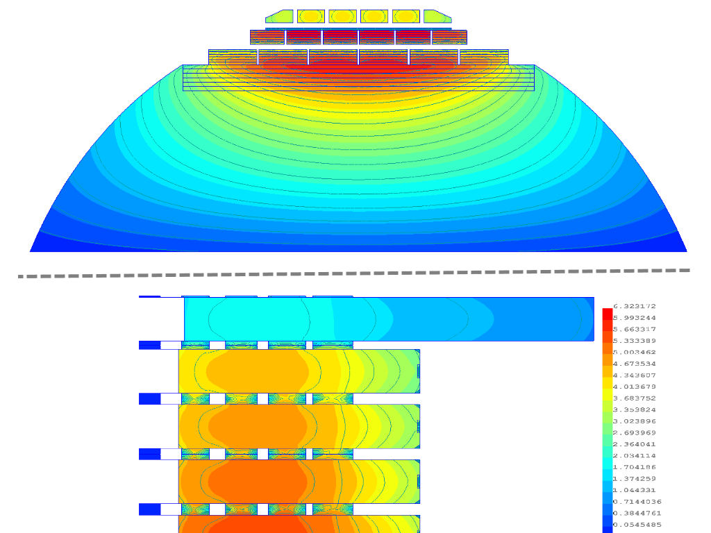
Postprocessor performs calculation results analysis (Fig. 5.1). Postprocessor allows to: draw field pattern as field lines and isotherms, obtain the pattern of different field values distribution, show local magnitudes of field values at any point of domain, draw field epures alone the given contours, compute contour integrals, surface integrals, and volume integrals.
Figure 5.1 Postprocessor window
Local values output
The 1 button switches on local values output mode (Fig. 5.1). At this mode output of field value magnitudes is carried out by pressing the left mouse button in the «Point values» dialog window (Fig. 5.2).
·Axisymmetric problem output values:
Title: Problem file name;
Coordinates: R, Z coordinates of the point which values are displayed;
Flux, Wb: magnetic flux flowing through the circle created by rotation of R,Z point around symmetry axis;
J, MA/m^2: density of total current at the point;
T, K: raise of point temperature above the ambient temperature;
Br, Bz, Tesla: R and Z components of magnetic flux density vector at the point;
|B|, Tesla: magnitude of magnetic flux density vector at the point;
Hr, Hz Amp/m: R and Z components of magnetic intensity at the point;
|H|, Amp/m: magnitude of magnetic intensity vector at the point;
Fr, Fz, Wt/K*m^2: R and Z components of heat flux vector;
|F|, Wt/K*m^2: magnitude of the heat flux vector;
P, W/m^3: resistive losses density;
Mu_r, Mu_z: R ans Z components of relative permeability;
E, J / m^3: magnetic field energy density;
dT/dr, dT/dz, K/m: R and Z components of temperature gradient vector;
grad(T), K/m: magnitude of the temperature gradient vector;
lambda_r, lambda_z, Wt/K*m: R and Z components of heat conductivity;
Q, Wt/K*m^3: heat power density;
- Plane problem output values:
Title: Problem file name;
Coordinates: X, Y coordinates of the point which values are displayed;
A, Wb/m: value of vector potential at the point;
J, MA/m^2: density of total current at the point;
T, K: raise of point temperature above the ambient temperature;
Bx, By, Tesla: X and Y components of magnetic flux density vector at the point;
|B|, Tesla: magnitude of the magnetic flux density vector;
Hx, Hy Amp/m: X and Y components of magnetic intensity vector at the point;
|H|, Amp/m: magnitude of the magnetic intensity vector;
Fx, Fy, Wt/K*m^2: X and Y components of heat flux vector;
|F|, Wt/K*m^2: magnitude of the heat flux vector;
P, W/m^3: resistive losses density;
Mu_x, Mu_y: X and Y components of relative permeability;
E, J / m^3: magnetic field energy density;
dT/dx, dT/dy, K/m: X and Y components of temperature gradient vector;
grad(T), K/m: magnitude of the temperature gradient vector;
lambda_x, lambda_y, Wt/K*m: X and Y components of heat conductivity;
Q, Wt/K*m^3: heat power density;
Figure 5.2 Local values at the point output window
Epure output
The program allows drawing epures along any given contour. Button 2 (Fig. 5.1) switches on contour edition mode. Contour is represented by piecewise-linear curve alone which different field values, surface and linear integrals are calculated. Pressing the left mouse button sets contour nodes. When dragging the mouse cursor with left button pressed contour marker arises. If the grid snap mode is on the contour node coincide with the nearest point of the geometry model or grid. Pressing the right mouse button deletes the contour.
Button 4 (Fig. 5.1) opens epures output window (Fig. 5.3). It is necessary to set the number of calculation point for composing the epure at the dialog window «Parameters of epures» in the «Number of points in epures» textbox.
Figure 5.3 Epures output window
When working with epures it is possible to pan the image by pressing the right mouse button and dragging the cursor at desirable direction, and to zoom the image by pressing the left mouse button and inscribing the necessary fragment into the frame.
Output epures:
A – Flux, Wb (Contour length, m): magnetic flux flowing through the circle created by rotation of the point around symmetry axis (concerns axisymmetric magnetic problem);
A – Magnetic vector potential, Wb/m (Contour length, m): distribution of magnetic potential vector along the contour; (concerns plane magnetic problem);
J total – Density of total current, A/m^2 (Contour length, m): destribution of current density along the contour;
B * n – Normal magnetic induction, Tesla (Contour length, m): normal magnetic flux density at the contour point;
B * t – Tangent magnetic induction, Tesla (Contour length, m): tangent magnetic flux density at the contour point;
|B | – Magnetic induction, Tesla (Contour length, m): magnitude of magnetic flux density vector at the contour point;
H * n – Normal intensity of magnetic field, A/m (Contour length, m): normal magnetic field intensity at the contour point;
H * t – Tangent intensity of magnetic field, A/m (Contour length, m): tangent magnetic field intensity at the contour point;
|H | – Intensity of magnetic field, A/m (Contour length, m): magnitude of magnetic field intensity vector at the contour point;
T – Temperature, K (Contour length, m): raise of the contour point temperature above the ambient medium temperature;
F * n – Normal heat flux, W/m^2 (Contour length, m): normal heat flux at the contour point;
F * t – Tangent heat flux, W/m^2 (Contour length, m): tangent heat flux at the contour point;
|F | – Heat flux, W/m^2 (Contour length, m): magnitude of the heat flux vector at the contour point;
Fn exp. – Normal heat flux, experimental, W/m^2 (Contour length, m): empirical dependence of normal heat flux upon tangent intensity of external magnetic field in the air at an edge of ferromagnetic (disregarding the influence of eddy currents in the ferromagnetic);
Derivation of contour, surface and volume integrals
In order to compute surface and contour integrals it is necessary to enter a contour (see item 5.2).
It order to compute volume integral it is necessary to select a volume of integration. Button 3 (Fig. 5.1) switches on (off) selection mode of the integration volume selection. At this mode pressing the left mouse button selects (deselects) the volume of the block the mouse cursor is pointing at. Pressing the right mouse button inverses volume selection.
Button 5 (Fig. 5.1) opens the «Contour integral» («Block integral») window in witch the necessary type of integral is selected.
Computation of contour and surface integrals
·Computation of contour integral for axisymmetric problem:
Average Current, A/m^2: contour average current;
Root-Mean-Square Current, A/m^2: contour root-mean-square current;
Bn:
Fn, Wb: normal magnetic flux flowing through the surface created by the contour revolution around the symmetry axis;
Bn, Tesla: average normal magnetic flux density at the surface created by the contour revolution around the symmetry axis;
Ht:
MMF, Amp-turns: contour magneto-motive force;
Ht, Amp/m: contour average tangent intensity of magnetic field;
Maxwell Force:
Steady-State Force, N: Maxwell’s force steady-state component;
2x Frequency Force, N: Maxwell’s force periodic (double-frequency) component (absent for the problems of magnetic field of direct currents calculation);
Temperature:
Maximum temperature, K: maximal temperature at the surface created by the contour revolution around the symmetry axis;
Average temperature, K: average temperature at the surface created by the contour revolution around the symmetry axis;
Heat Flow:
P, W: heat power flowing through the surface created by the contour revolution around the symmetry axis;
Average Heat Flow, W/m^2: normal average heat flow at the surface created by the contour revolution around symmetry axis;
Contour length, m: contour length;
·Computation of contour integrals for plane problem:
Average Current, A/m^2: contour average current;
Root-Mean-Square Current, A/m^2: contour root-mean-square current;
Bn:
Fn, Wb: normal magnetic flux though the surface created by extruding of the contour along Z axis with the depth «Bodies Depth, mm» (see item 4.2.1);
Bn, Tesla: average normal magnetic flux density at the surface created by extruding of the contour along Z axis with the length «Bodies Depth, mm»;
Ht:
MMF, Amp-turns: magneto-motive force along the contour;
Ht, Amp/m: average tangent intensity of the magnetic field along the contour;
Maxwell Force:
Steady-State Force, N: Maxwell’s force steady-state component;
2x Frequency Force, N: Maxwell’s force periodic (double-frequency) component (absent for the problems of magnetic field of direct currents calculation);
Temperature:
Maximum temperature, K: maximal temperature at the surface created by extruding of the contour along Z axis with the length «Bodies Depth, mm»;
Average temperature, K: average temperature at the surface created by extruding of the contour along Z axis with the length «Bodies Depth, mm»;
Heat Flow:
P, W: heat power flowing through the surface created by extruding of the contour along Z axis with the length «Bodies Depth, mm»;
Average Heat Flow, W/m^2: normal average heat flow at the surface created by extruding of the contour along Z axis with the length «Bodies Depth, mm»;
Contour length, m: contour length;
Computation of volume integrals
Temperature, K:
Maximum temperature, K: maximum temperature in the selected volume;
Average temperature, K: average temperature in the selected volume;
A.J, H*A^2: Self-inductance is calculated using this integral. Contour self-inductance is found as A.J integral divided by squared pick value of the current in the contour.
A, H*A: volume average magnetic field flux. The integral is used to calculate mutual inductance of two contours. Two contours mutual inductance is found as average flux flowing through the first contour divided by value of the current in the second contour provided the first contour is de-energized.
Resistive losses, W: resistance losses in the selected volume;
Integral of B over block, Tesla: R, Z (X, Y) components of volume average magnetic flux density;
Total Current, A: total current flowing through the selected section;
Lorentz Force, N:
Steady-State Force, N: Lorentz force steady-state component;
2x Frequency Force, N: Lorentz force periodic (double-frequency) component (absent for the problems of magnetic field of direct currents calculation);
Energy of magnetic field, J: energy of the magnetic field in the selected volume. For the problems of direct currents magnetic field calculation the field energy is found as:
Heat power, W: heat power emitted in the volume;
Block cross-section area, m^2: area of the selected section;
Block volume, m^3: volume of the selected domain;